Chart Styles and Layouts - M. S. Excel Tutorials - Science Tutor

Chart Styles and Layouts

You can easily change the Style of your chart. If you can't see the Styles, click anywhere on your chart to select it, and you should see the Ribbon change. The Styles will look like this in Excel 2007:

In later versions of Excel, your Chart Styles will look like this:

Click on any chart style, and your chart will change. To see more styles, click the arrows to the right of the Chart Styles panel:

You'll then see a drop down sheet of new styles (Excel 2007):

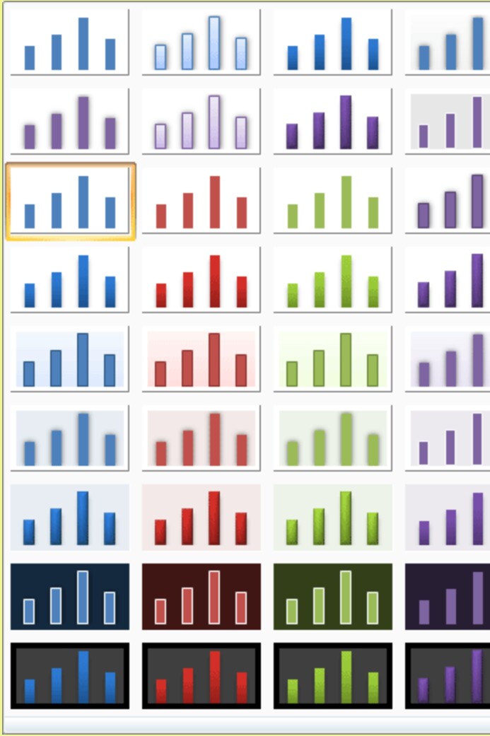
And here's the Styles in Excel 2013:

Work your way through the Styles, and click on each one in turn. Watch what happens to your chart when you select a style.

 

Chart Layouts

You can also change the layout of your chart in the same way. Locate the Chart Layoutpanel on the Design tab of the Excel Ribbon bar. It looks like this in Excel 2007: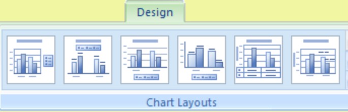

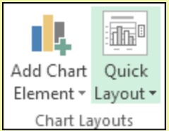
In later versions you may have to click theQuick Layout option on the Chart Layoutspanel:

Click the down arrow to the right of the Chart Layouts panel to see the available layouts you can choose from:

Again, click on each one in turn and see what happens to your chart. In the image below, we've gone for Layout 10:

Changing the Chart Type - 2D Bar Charts

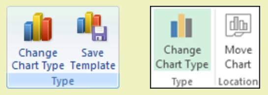
You can change the type of chart, as well. Instead of having a 2D column chart, as above, you can have a 2D bar chart. To change the chart type, locate the Type panel on the Excel Ribbon bar (you need to have your chart selected to see it):

        

Then click Change Chart Type. You'll see a dialogue box appear. This one is from Excel 2007:

The dialogue box looks slightly different in Excel 2013:

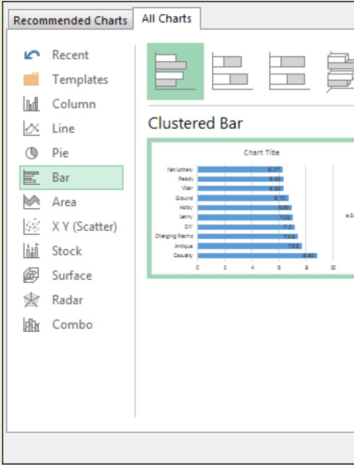
Select Bar from the list on the left of the dialogue box, and click on the first Bar chart (Clustered Bar). Click OK to see your chart change:

You can experiment with the types of chart in the dialogue box. But reset it to Bar chart, as above.

In the next part, you'll see how to format a chart, so that you can change the Series 1 and Chart Title headings.