Science Tutor

The Statue of Unity

Anoop Kumar Sharma October 31, 2018

The Statue of Unity

The Statue of Unity is the world's tallest statue monument. The statue is located on the river island called Sadhu Bet facing the Narmada Dam near Rajpipla in Indian state of Gujarat.

The Statue of Unity is the world's tallest statue monument of 182 meters. Statue of Unity is dedicated to the sculptor of modern India, viz., the first deputy Prime Minister of India and Bharat Ratna Sardar Vallabhbhai Patel. Sardar Vallabhbhai Patel, also known as the Iron Man of India.

The Statue of Unity

Reviewed by Anoop Kumar Sharma on October 31, 2018 Rating: 5

Meaning & Full Form of "Ft."

Anoop Kumar Sharma October 28, 2018

Meaning & Full Form of "Ft."

It's short for ‘featuring’, and also is sometimes written as “feat.”. Seen with another artist's (or multiple featuring artists') name, for example;

“Honey Sing - Song ft. Dr. Zeus”.

In which Honey Singh is the main artist of ‘Song' and Dr. Zeus is a featuring artist, often having a shorter part in the song than the main artist.

Meaning & Full Form of "Ft."

Reviewed by Anoop Kumar Sharma on October 28, 2018 Rating: 5

CountIF - Formula in M. S. Excel - Science Tutor

Anoop Kumar Sharma October 22, 2018

Another useful function that uses Conditional Logic is CountIF. This one is fairly straightforward. As its name suggests, it counts things! But it counts things IF a condition is met. For example, keep a count of how many students have an A Grade.

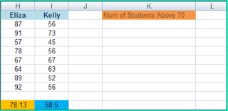
To get you started with this function, we'll use our and count how many students have a score of 70 or above. First, add the following label to your spreadsheet:

As you can see, we've put our new label at the start of the K column.

We can now use the CountIF function to see how many of the students scored 70 or above for a given subject.
The CountIF function looks like this:

COUNTIF(range, criteria)

The function takes two arguments (the words in the round brackets). The first argument is range, and this means the range of cells you want Excel to count. Criteria means, "What do you want Excel to look for when it's counting?".
So click inside cell K2, and then click inside the formula bar at the top. Enter the following formula:

=CountIf(B2:I2, ">= 70")

The cells B2 to I2 contain the Math scores for all 8 students. It's these scores we want to count.
Press the enter key on your keyboard. Excel should give you an answer of 4:

(If you're wondering where the columns B to I have gone in the image above, we've hidden then for convenience sake!)

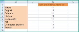
To do the rest of the scores, you can use AutoFill. You should then have a K column that looks like this:

By using CountIF, we can see at a glance which subjects students are doing well in, and which subjects they are struggling in.

Exercise
Add a new label to the L column. In the cells L2 to L9, work out how many students got below 50 for a given subject. You should get the same results as in the image below:

CountIF - Formula in M. S. Excel - Science Tutor

Reviewed by Anoop Kumar Sharma on October 22, 2018 Rating: 5

Conditional Formatting in Excel 2007/2010 - M. S. Excel Tutorials - Science Tutor

Anoop Kumar Sharma October 09, 2018

You can use something called Conditional Formatting in your Excel spreadsheets. Conditional Formatting allows you to change the appearance of a cell, depending on certain conditions. What we'll do is to colour the Overall Averages on our Student Exam spreadsheet, depending on the grade. Here's the spreadsheet we'll be working on.

Open up your Student Exam spreadsheet (You did complete it, didn't you?)
Highlight the cells with Overall Grades, which should be cells B11 to I11

The Overall Averages range from 44 to 85. We'll colour each grade, depending on a scale. A different colour will apply to the following grades:

50 and below
51 to 60
61 to 70
71 to 80
81 and above

So five different bands, and a colour for each. To set the Conditional Formatting in Excel, do the following:

With your Overall Averages highlighted, click on the Home menu at the top of Excel
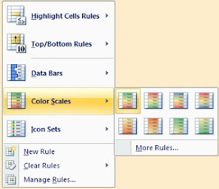
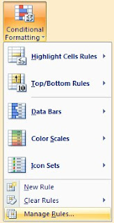
Locate the Styles panel, and the Conditional Formatting item:

The Conditional Formatting menu gives you various options. The easiest one is the Colour Scales option. Select one of these and Excel will colour the cell backgrounds for you:

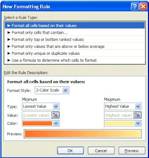
That's not quite what we're looking for, though. We'd like to choose our own values. So click on More Rules, from the Colour Scales submenu. You'll see the following rather complex dialogue box:

The one we want is the second option, Format only cells that contain. This will allow us to set up our values. When you click this option, the dialogue box changes to this:

The part we're interested in is the bottom part, under the heading Edit the Rule Description. It says Cell Value and Between, in the drop down boxes. These are the ones we want. We only need to type a value for the two boxes that are currently blank in the image above. We can then click the Format button to choose a colour.

So type 0 in the first box and 50 in the second one:

Then click the Format button. You'll get another dialogue box popping up. This is just the Format Cells one though. You've met this before. Click on the Fill tab and choose a colour. Click OK and you should see something like this under Edit the Rule Description:

The Preview is showing the colour we picked. So we've said, "If the Cell Value is between 0 and 50 then colour the cell Red".
Click OK on this dialogue box to get back to Excel. You should find that one of the cells has turned red. To format the rest of the cells, click on Conditional Formatting on the Styles panel again. From the menu, click on Manage Rules:

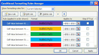
You'll get yet another complex dialogue box popping up! This one:

Our first rule is already there - Cell Value Between. The only thing we're doing here is adding New Rules, similar to the one we've just set up. Click the New Rule button then. You'll see the exact same dialogue boxes you used to set up the first rule. Set a new colour for the next scores - 51 to 60. Choose a colour, and keep clicking OK until you get back to the Rules Manager dialogue box. It should now look something like this one:

We now have to colours in our range. Do the rest of the scores, choosing a colour for each. The scores are these, remember:

50 and below
51 to 60
61 to 70
71 to 80
81 and above

When you've done them all, your dialogue box should have five colours:

The colours above are entirely arbitrary, and you don't have to select the same ones we did. The point is to have a different colour for each range of scores. But click OK when you're done. Your Overall Averages will then look something like this:

Formatting your spreadsheet in this way allows you to see at a glance relevant information. In the spreadsheet above, it's obvious who's failing - just look for the red cells!

In the next part, we'll look at a useful function that counts things - COUNT IF.

Buy Complete M.S. Excel Tutorial Book From Amazon : https://amzn.to/2yEYXgk