Review Number One - M. S. Excel Tutorials - Science Tutor

Reviewed by
Anoop Kumar Sharma
on
July 27, 2018
Rating:
5
How to Merge Cells - M. S. Excel Tutorials - Science Tutor

Reviewed by
Anoop Kumar Sharma
on
July 27, 2018
Rating:
5
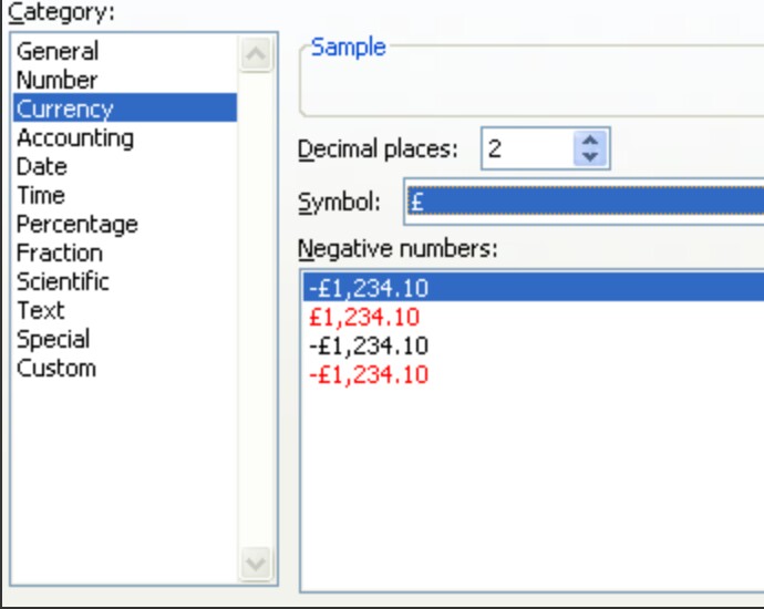
Currency Symbols in Excel 2007/2010 - M. S. Excel Tutorials - Science Tutor

Reviewed by
Anoop Kumar Sharma
on
July 27, 2018
Rating:
5
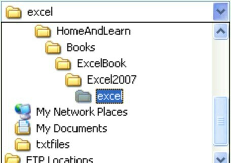
How to Save your work in Excel - M. S. Excel Tutorials - Science Tutor

Reviewed by
Anoop Kumar Sharma
on
July 26, 2018
Rating:
5
How to change the colour of a Cell - M. S. Excel Tutorials - Science Tutor

Reviewed by
Anoop Kumar Sharma
on
July 25, 2018
Rating:
5
Font Formatting in Excel 2007/2010 - M. S. Excel Tutorials - Science Tutor

Reviewed by
Anoop Kumar Sharma
on
July 23, 2018
Rating:
5
How to Centre text and numbers - M. S. Excel Tutorials - Science Tutor

Reviewed by
Anoop Kumar Sharma
on
July 23, 2018
Rating:
5
How to Edit text in a Cell - M. S. Excel Tutorials - Science Tutor

Reviewed by
Anoop Kumar Sharma
on
July 13, 2018
Rating:
5
Enter text and numbers in a Cell - M.S. Excel Tutorials - Science Tutor

Reviewed by
Anoop Kumar Sharma
on
July 09, 2018
Rating:
5